How to Sort in Excel: A Simple Guide to Organizing Data

When it comes to Excel, here's a good rule to live by: If you find yourself doing something manually, there's probably an easier way.

Whether you're trying to remove duplicates, do simple calculations, or sort your data, you can almost always find a workaround that'll help you get it done with just a click (or two) of a button.

But if you're not a power user, it's easy to overlook these shortcuts. And before you know it, something as simple as organizing a list of names in alphabetical order can suck up a ton of your time.

Luckily, there is a workaround for that. In fact, there are a few different ways to use Excel's sorting feature that you may not know about. Let's check them out below, starting with the basics.

How to Sort in Excel

1. Highlight the rows and/or columns you want sorted.
2. Navigate to "Data" along the top and select "Sort."
3. If sorting by column, select the column you want to order your sheet by.
4. If sorting by row, click "Options" and select "Sort left to right."
5. Choose what you'd like sorted.
6. Choose how you'd like to order your sheet.
7. Click "OK."

For this first set of instructions, we'll be using Microsoft Excel 2017 for Mac. But don't worry -- while the location of certain buttons might be different, the icons and selections you have to make are the same across most earlier versions of Excel.

1. Highlight the rows and/or columns you want sorted.

To sort a range of cells in Excel, first click and drag your cursor across your spreadsheet to highlight all of the cells you want to sort -- even those rows and columns whose values you're not actually sorting by.

For example, if you want to sort column A, but there's data associated with column A in columns B and C, it's important to highlight all three columns to ensure the values in Columns B and C move along with the cells you're sorting in Column A.

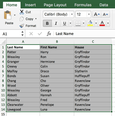
In the screenshot below, we're going to sort this sheet by the last name of Harry Potter characters. But the first name and house of each person needs to go with each last name that gets sorted, or each column will become mismatched when we finish sorting.

2. Navigate to 'Data' along the top and select 'Sort.'

Once all the data you want to sort is highlighted, select the "Data" tab along the top navigation bar (you can see this button on the top-right of the screenshot in the first step, above). This tab will expand a new set of options beneath it, where you can select the "Sort" button. The icon has an "A-Z" graphic on it, as you can see below, but you'll be able to sort in more ways than just alphabetically.

3. If sorting by column, select the column you want to order your sheet by.

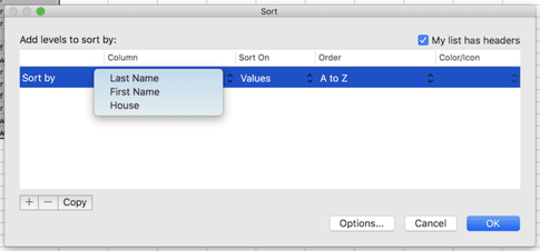
When you hit the "Sort" button, shown above, a window of settings will appear. This is where you can configure what you'd like sorted and how you'd like to sort it.

If you're sorting by a specific column, click "Column" -- the leftmost dropdown menu, shown below -- and select the column whose values you want to be your sorting criteria. In our case, it'll be "Last Name."

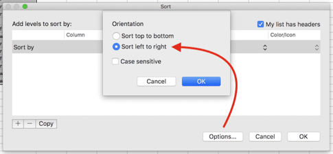
4. If sorting by row, click 'Options' and select 'Sort left to right.'

If you'd rather sort by a specific row, rather than a column, click "Options" on the bottom of the window and select "Sort left to right." Once you do this, the Sort settings window will reset and ask you to choose the specific "Row" you'd like to sort by in the leftmost dropdown (where it currently says "Column").

This sorting system doesn't quite make sense for our example, so we'll stick with sorting by the "Last Name" column.

5. Choose what you'd like sorted.

You don't just have to sort by the value of each cell. In the middle column of your Sort settings window, you'll see a dropdown menu called "Sort On." Click it, and you can choose to sort your sheet by different characteristics of each cell in the column/row you're sorting by. These options include cell color, font color, or any icon included in the cell.

6. Choose how you'd like to order your sheet.

In the third section of your Sort settings' window, you'll see a dropdown bar called "Order." Click it to select how you'd like to order your spreadsheet.

By default, your Sort settings window will suggest sorting alphabetically (which we'll show you shortcuts for in the next process below). But you can also sort from Z to A, as well as by a custom list. While you can create your own custom list, there are a few preset lists you can sort your data by right away. We'll talk more about how and why you might sort by custom list in a few minutes.

To Sort by Number

If your spreadsheet includes a column of numbers, rather than letter-based values, you can also sort your sheet by these numbers. To do that, you'll select this column in the leftmost "Columns" dropdown menu. This will change the options in the "Order" dropdown bar so that you can sort from "Smallest to Largest" or "Largest to Smallest."

7. Click 'OK.'

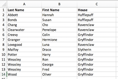
Click "OK," in your Sort settings window, and you should see your list successfully sorted according to your desired criteria. Here's what our Harry Potter list now looks like, organized by last name in alphabetical order:

How to Alphabetize in Excel

To alphabetize in Excel, highlight a cell in the column you want to sort by. Click the Data tab along the top navigation, and you'll see buttons for sorting in forward or reverse alphabetical order. Clicking either button will order your sheet according to the column of the cell you first highlighted.

Sometimes you may have a list of data that has no organization whatsoever. Maybe you exported a list of your marketing contacts or blog posts. Whatever the case may be, you might want to start by alphabetizing the list -- and there's an easy way to do this that doesn't require you to follow each step outlined above.

To Alphabetize on a Mac

1. Select a cell in the column you want to sort.
2. Click on the "Data" tab in your toolbar and look for the "Sort" option on the left.
3. If the "A" is on top of the "Z," you can just click on that button once. If the "Z" is on top of the "A," click on the button twice. Note: When the "A" is on top of the "Z," that means your list will be sorted in alphabetical order. However, when the "Z" is on top of the "A," that means your list will be sorted in reverse alphabetical order.

To Alphabetize on a PC

1. Select a cell in the column you want to sort.
2. Click on the "Data" tab in your toolbar. You will see Sort options in the middle.
3. Click on the icon above the word "Sort." A pop-up will appear: If you have headers, make sure "My list has headers" is checked. If it is, click "Cancel."
4. Click on the button that has the "A" on top and the "Z" on the bottom with an arrow pointing down. That will sort your list alphabetically from "A" to "Z." If you want to sort your list in reverse alphabetical order, click on the button that has the "Z" on top and the "A" on the bottom.

Sorting Multiple Columns

Sometimes you don't just want to sort one column, but you want to sort two. Let's say you want to organize all of your blog posts that you have in a list by the month they were published. First, you'd want to organize them by date, and then by the blog post title or URL.

In this example, I want to sort my list first by house, and then by last name. This would give me a list organized by each house, but also alphabetized within each house.

To Sort Multiple Columns on a Mac

1. Click on the data in the column you want to sort.
2. Click on the "Data" tab in your toolbar and look for the "Sort" option on the left.
3. Click on the small arrow to the left of the "A to Z" Sort icon. Then, select "Custom Sort" from the menu.
4. A pop-up will appear: If you have headers, make sure "My list has headers" is checked.
5. You will see five columns. Under "Column" select the first column you want to sort from the dropdown menu. (In this case, it is "House.")
6. Then, click on the "+" sign at the bottom left of the pop-up. Under where it says "Column," select "Last Name" from the dropdown.
7. Check the "Order" column to make sure it says A to Z. Then click "OK."
8. Marvel at your beautiful organized list.

To Sort Multiple Columns on a PC

1. Click on the data in the column you want to sort.
2. Click on the "Data" tab in your toolbar. You will see "Sort" options in the middle.
3. Click on the icon above the word "Sort." You will see a pop-up appear. Make sure "My data has headers" is checked if you have column headers.
4. You will see three columns. Under "Column" select the first column you want to sort from the dropdown menu. (In this case, it is "House.")
5. Then click on "Add Level" at the top left of the pop-up. Under where it says "Column" select "Last Name" from the dropdown.
6. Check the "Order" column to make sure it says A to Z. Then click "OK."
7. Marvel at your beautiful organized list.

Sorting in Custom Order

Sometimes you don't want to sort by A to Z or Z to A. Sometimes you want to sort by something else, such as months, days of the week, or some other organizational system.

In situations like this, you can create your own custom order to specify exactly the order you want the sort. (It follows a similar path to multiple columns but is slightly different.)

Let's say we have everyone's birthday month at Hogwarts, and we want everyone to be sorted first by Birthday Month, then by House, and then by Last Name.

To Sort in Custom Order on a Mac

1. Click on the data in the column you want to sort.
2. Click on the "Data" tab in your toolbar. You will see "Sort" all the way to the left.
3. Click on the small arrow to the left of the "A to Z" Sort icon. Then, select "Custom Sort" from the menu.
4. A pop-up will appear: If you have headers, make sure "My list has headers" is checked.
5. You will see five columns. Under "Column," select the first column in your spreadsheet you want to sort from the dropdown menu. In this case, it is "Birthday Month."
6. Under the "Order" column, click on the dropdown next to "A to Z." Select the option for "Custom List."
7. You will see a couple of options (month and day). Select the month list where the months are spelled out, as that matches the data. Click "OK."
8. Then click on the "+" sign at the bottom left of the pop-up. Under "Column," select "House" from the dropdown.
9. Click on the "+" sign at the bottom left again. Under "Column," select "Last Name" from the dropdown.
10. Check the "Order" column to make sure "House" and "Last Name" say A to Z. Then click "OK."
11. Marvel at your beautiful organized list.

To Sort in Custom Order on a PC

1. Click on the data in the column you want to sort.
2. Click on the "Data" tab in your toolbar. You will see "Sort" options in the middle.
3. Click on the icon above the word "Sort." You will see a pop-up appear: If you have headers, make sure "My list has headers" is checked.
4. You will see three columns. Under "Column," select the first column you want to sort from the dropdown. In this case, it is "Birthday Month."
5. Under the "Order" column, click on the dropdown next to "A to Z." Select the option for "Custom List."
6. You will see a couple of options (month and day), as well as the option to create your own custom order. Select the month list where the months are spelled out, as that matches the data. Click "OK."
7. Then, click on "Add Level" at the top left of the pop-up. Under "Column," select "House" from the dropdown.
8. Click on the "Add Level" button at the top left of the pop-up again. Under "Column," select "Last Name" from the dropdown.
9. Check the "Order" column to make sure "House" and "Last Name" say A to Z. Then click "OK."
10. Marvel at your beautiful organized list.

Sorting a Row

Sometimes your data may appear in rows instead of columns. When that happens you are still able to sort your data with a slightly different step.

To Sort a Row on a Mac

1. Click on the data in the row you want to sort.
2. Click on the "Data" tab in your toolbar. You will see "Sort" all the way to the left.
3. Click on the small arrow to the left of the "A to Z" Sort icon. Then, select "Custom Sort" from the menu.
4. A pop-up will appear: Click on "Options" at the bottom.
5. Under "Orientation" select "Sort left to right." Then, click "OK."
6. You will see five columns. Under "Row," select the row number that you want to sort from the dropdown. (In this case, it is Row 1.) When you are done, click "OK."

To Sort a Row on a PC

1. Click on the data in the row you want to sort.
2. Click on the "Data" tab in your toolbar. You will see "Sort" options in the middle.
3. Click on the icon above the word "Sort." You will see a pop-up appear.
4. Click on "Options" at the bottom.
5. Under "Orientation" select "Sort left to right." Then, click "OK."
6. You will see three columns. Under "Row," select the row number that you want to sort from the dropdown. (In this case, it is Row 1.) When you are done, click "OK."

Sort Your Conditional Formatting

If you use conditional formatting to change the color of a cell, add an icon, or change the color of a font, you can actually sort by that, too.

In the example below, I've used colors to signify different grade ranges: If they have a 90 or above, the cell appears green. Between 80-90 is yellow. Below 80 is red. Here's how you'd sort that information to put the top performers at the top of the list. I want to sort this information so that the top performers are at the top of the list.

To Sort Conditional Formatting on a Mac

1. Click on the data in the row you want to sort.
2. Click on the "Data" tab in your toolbar. You will see "Sort" all the way to the left.
3. Click on the small arrow to the left of the "A to Z" Sort icon. Then, select "Custom Sort" from the menu.
4. A pop-up will appear: If you have headers, make sure "My list has headers" is checked.
5. You will see five columns. Under "Column," select the first column you want to sort from the dropdown. In this case, it is "Grades."
6. Under the column that says "Sort On," select "Cell Color".
7. In the last column that says "Color/Icon," select the green bar.
8. Then click on the "+" sign at the bottom left of the pop-up. Repeat steps 5-6. Instead of selecting green under "Color/Icon," select the yellow bar.
9. Then click on the "+" sign at the bottom left of the pop-up. Repeat steps 5-6. Instead of selecting green under "Color/Icon," select the red bar.
10. Click "OK."

To Sort Conditional Formatting on a PC

1. Click on the data in the row you want to sort.
2. Click on the "Data" tab in your toolbar. You will see "Sort" options in the middle.
3. Click on the icon above the word "Sort." A pop-up will appear: If you have headers, make sure "My list has headers" is checked.
4. You will see three columns. Under "Column" select the first column you want to sort from the dropdown. In this case, it is "Grades."
5. Under the column that says "Sort On," select "Cell Color".
6. In the last column that says "Order," select the green bar.
7. Click on "Add Level." Repeat steps 4-5. Instead of selecting green under "Order," select the yellow bar.
8. Click on "Add Level" again. Repeat steps 4-5. Instead of selecting yellow under "Order," select the red bar.
9. Click "OK."

There you have it -- all the possible ways to sort in Excel. Ready to sort your next spreadsheet? Start by grabbing nine different Excel templates below, then use Excel's sorting function to organize your data as you see fit.

from Marketing https://blog.hubspot.com/marketing/how-to-sort-in-excel