24 Excel Formulas, Keyboard Shortcuts & Tricks That'll Save You Lots of Time

Marketing and Microsoft Excel go together like peanut butter and chocolate. There's just one problem.

For many of us, trying to organize and analyze Excel worksheets can feel like walking into a brick wall over and over again. You're manually replicating columns and scribbling down long-form math on a scrap of paper, all while thinking to yourself, "There has to be a better way to do this."

Truth be told, there is -- you just don't know it yet.

Excel can be tricky that way. On one hand, it's an exceptionally powerful tool for reporting and analyzing marketing data. On the other, without the proper training, it's easy to feel like it's working against you. For starters, there are more than a dozen critical formulas Excel can automatically run for you so you're not combing through hundreds of cells with a calculator on your desk.

Excel Formulas

1. IF
2. Percentage
3. Subtraction
4. Multiplication
5. Division
6. DATE
7. Array
8. COUNT
9. AVERAGE
10. SUMIF
11. TRIM
12. LEFT, MID, and RIGHT
13. VLOOKUP
14. RANDOMIZE

To help you use Excel more effectively (and save a ton of time), we've compiled a list of essential formulas, keyboard shortcuts, and other small tricks and functions you should know.

NOTE: The following formulas apply to Excel 2017. If you're using a slightly older version of Excel, the location of each feature mentioned below might be slightly different.

IF Formula in Excel

The IF formula in Excel is denoted =IF(logical_test, value_if_true, value_if_false). This allows you to enter a text value into the cell "if" something else in your spreadsheet is true or false. For example, =IF(D2="Gryffindor","10","0") would award 10 points to cell D2 if that cell contained the word "Gryffindor."

There are times when we want to know how many times a value appears in our spreadsheets. But there are also those times when we want to find the cells that contain those values, and input specific data next to it.

We'll go back to Sprung's example for this one. If we want to award 10 points to everyone who belongs in the Gryffindor house, instead of manually typing in 10's next to each Gryffindor student's name, we'll use the IF-THEN formula to say: If the student is in Gryffindor, then he or she should get ten points.

• The formula: IF(logical_test, value_if_true, value_if_false)
  • Logical_Test: The logical test is the "IF" part of the statement. In this case, the logic is D2="Gryffindor." Make sure your Logical_Test value is in quotation marks.
  • Value_if_True: If the value is true -- that is, if the student lives in Gryffindor -- this value is the one that we want to be displayed. In this case, we want it to be the number 10, to indicate that the student was awarded the 10 points. Note: Only use quotation marks if you want the result to be text instead of a number.
  • Value_if_False: If the value is false -- and the student does not live in Gryffindor -- we want the cell to show "0," for 0 points.
• Formula in below example: =IF(D2="Gryffindor","10","0")

Percentage Formula in Excel

To perform the percentage formula in Excel, enter the cells you're finding a percentage for in the format, =A1/B1. To convert the resulting decimal value to a percentage, highlight the cell, click the Home tab, and select "Percentage" from the numbers dropdown.

There isn't an Excel "formula" for percentages per se, but Excel makes it easy to convert the value of any cell into a percentage so you're not stuck calculating and reentering the numbers yourself.

The basic setting to convert a cell's value into a percentage is under Excel's Home tab. Select this tab, highlight the cell(s) you'd like to convert to a percentage, and click into the dropdown menu next to Conditional Formatting (this menu button might say "General" at first). Then, select "Percentage" from the list of options that appears. This will convert the value of each cell you've highlighted into a percentage. See this feature below.

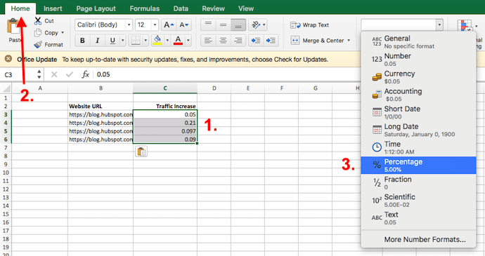
Keep in mind if you're using other formulas, such as the division formula (denoted =A1/B1), to return new values, your values might show up as decimals by default. Simply highlight your cells before or after you perform this formula, and set these cells' format to "Percentage" from the Home tab -- as shown above.

Subtraction Formula in Excel

To perform the subtraction formula in Excel, enter the cells you're subtracting in the format, =SUM(A1, -B1). This will subtract a cell using the SUM formula by adding a negative sign before the cell you're subtracting. For example, if A1 was 10 and B1 was 6, =SUM(A1, -B1) would perform 10 + -6, returning a value of 4.

Like percentages, subtracting doesn't have its own formula in Excel either, but that doesn't mean it can't be done. You can subtract any values (or those values inside cells) two different ways.

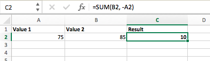
• Using the =SUM formula. To subtract multiple values from one another, enter the cells you'd like to subtract in the format =SUM(A1, -B1), with a negative sign (denoted with a hyphen) before the cell whose value you're subtracting. Press enter to return the difference between both cells included in the parentheses. See how this looks in the screenshot above.
• Using the format, =A1-B1. To subtract multiple values from one another, simply type an equals sign followed by your first value or cell, a hyphen, and the value or cell you're subtracting. Press Enter to return the difference between both values.

Multiplication Formula in Excel

To perform the multiplication formula in Excel, enter the cells you're multiplying in the format, =A1*B1. This formula uses an asterisk to multiply cell A1 by cell B1. For example, if A1 was 10 and B1 was 6, =A1*B1 would return a value of 60.

You might think multiplying values in Excel has its own formula or uses the "x" character to denote multiplication between multiple values. Actually, it's as easy as an asterisk -- *.

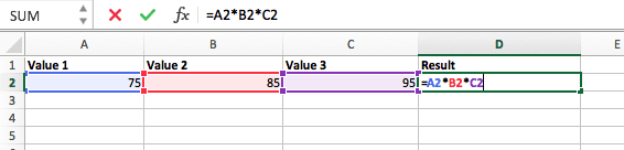
To multiply two or more values in an Excel spreadsheet, highlight an empty cell. Then, enter the values or cells you want to multiply together in the format, =A1*B1*C1 ... etc. The asterisk will effectively multiply each value included in the formula.

Press Enter to return your desired product. See how this looks in the screenshot above.

Excel Division Formula

To perform the division formula in Excel, enter the cells you're dividing in the format, =A1/B1. This formula uses a forward slash, "/," to divide cell A1 by cell B1. For example, if A1 was 5 and B1 was 10, =A1/B1 would return a decimal value of 0.5.

Division in Excel is one of the simplest functions you can perform. To do so, highlight an empty cell, enter an equals sign, "=," and follow it up with the two (or more) values you'd like to divide with a forward slash, "/," in between. The result should be in the following format: =B2/A2, as shown in the screenshot below.

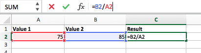
Hit Enter, and your desired quotient should appear in the cell you initially highlighted.

Excel DATE Formula

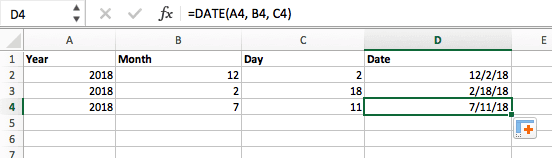
The Excel DATE formula is denoted =DATE(year, month, day). This formula will return a date that corresponds to the values entered in the parentheses -- even values referred from other cells. For example, if A1 was 2018, B1 was 7, and C1 was 11, =DATE(A1,B1,C1) would return 7/11/2018.

Creating dates in the cells of an Excel spreadsheet can be a fickle task every now and then. Luckily, there's a handy formula to make formatting your dates easy. There are two ways to use this formula:

• Create dates from a series of cell values. To do this, highlight an empty cell, enter "=DATE," and in parentheses, enter the cells whose values create your desired date -- starting with the year, then the month number, then the day. The final format should look like this: =DATE(year, month, day). See how this looks in the screenshot below.
• Automatically set today's date. To do this, highlight an empty cell and enter the following string of text: =DATE(YEAR(TODAY()), MONTH(TODAY()), DAY(TODAY())). Pressing enter will return the current date you're working in your Excel spreadsheet.

In either usage of Excel's date formula, your returned date should be in the form of "mm/dd/yy" -- unless your Excel program is formatted differently.

Excel Array Formula

An array formula in Excel surrounds a simple formula in brace characters using the format, {=(Start Value 1:End Value 1)*(Start Value 2:End Value 2)}. By pressing ctrl+shift+center, this will calculate and return value from multiple ranges, rather than just individual cells added to or multiplied by one another.

Calculating the sum, product, or quotient of individual cells is easy -- just use the =SUM formula and enter the cells, values, or range of cells you want to perform that arithmetic on. But what about multiple ranges? How do you find the combined value of a large group of cells?

Numerical arrays are a useful way to perform more than one formula at the same time in a single cell so you can see one final sum, difference, product, or quotient. If you're looking to find total sales revenue from several sold units, for example, the array formula in Excel is perfect for you. Here's how you'd do it:

1. To start using the array formula, type "=SUM," and in parentheses, enter the first of two (or three, or four) ranges of cells you'd like to multiply together. Here's what your progress might look like: =SUM(C2:C5
2. Next, add an asterisk after the last cell of the first range you included in your formula. This stands for multiplication. Following this asterisk, enter your second range of cells. You'll be multiplying this second range of cells by the first. Your progress in this formula should now look like this: =SUM(C2:C5*D2:D5)
3. Ready to press Enter? Not so fast ... Because this formula is so complicated, Excel reserves a different keyboard command for arrays. Once you've closed the parentheses on your array formula, press Ctrl+Shift+Enter. This will recognize your formula as an array, wrapping your formula in brace characters and successfully returning your product of both ranges combined.

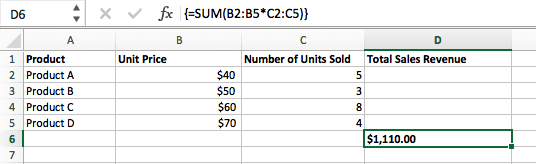
In revenue calculations, this can cut down on your time and effort significantly. See the final formula in the screenshot below.

COUNT Formula in Excel

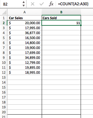
The COUNT formula in Excel is denoted =COUNT(Start Cell:End Cell). This formula will return a value that is equal to the number of entries found within your desired range of cells. For example, if there are eight cells with entered values between A1 and A10, =COUNT(A1:A10) will return a value of 8.

The COUNT formula in Excel is particularly useful for large spreadsheets, wherein you want to see how many cells contain actual entries. Don't be fooled: This formula won't do any math on the values of the cells themselves. This formula is simply to find out how many cells in a selected range are occupied with something.

Using the formula in bold above, you can easily run a count of active cells in your spreadsheet. The result will look a little something like this:

AVERAGE Formula in Excel

To perform the average formula in Excel, enter the values, cells, or range of cells of which you're calculating the average in the format, =AVERAGE(number1, number2, etc.) or =AVERAGE(Start Value:End Value). This will calculate the average of all the values or range of cells included in the parentheses.

Finding the average of a range of cells in Excel keeps you from having to find individual sums and then performing a separate division equation on your total. Using =AVERAGE as your initial text entry, you can let Excel do all the work for you.

For reference, the average of a group of numbers is equal to the sum of those numbers, divided by the number of items in that group.

SUMIF Formula in Excel

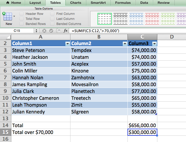
The SUMIF formula in Excel is denoted =SUMIF(range, criteria, [sum range]). This will return the sum of the values within a desired range of cells that all meet one criterion. For example, =SUMIF(C3:C12,">70,000") would return the sum of values between cells C3 and C12 from only the cells that are greater than 70,000.

Let's say you want to determine the profit you generated from a list of leads who are associated with specific area codes, or calculate the sum of certain employees' salaries -- but only if they fall above a particular amount. Doing that manually sounds a bit time-consuming, to say the least.

With the SUMIF function, it doesn't have to be -- you can easily add up the sum of cells that meet certain criteria, like in the salary example above.

• The formula: =SUMIF(range, criteria, [sum_range])
  
  • Range: The range that is being tested using your criteria.
  • Criteria: The criteria that determine which cells in Criteria_range1 will be added together
  • [Sum_range]: An optional range of cells you're going to add up in addition to the first Range entered. This field may be omitted.

In the example below, we wanted to calculate the sum of the salaries that were greater than $70,000. The SUMIF function added up the dollar amounts that exceeded that number in the cells C3 through C12, with the formula =SUMIF(C3:C12,">70,000").

TRIM Formula in Excel

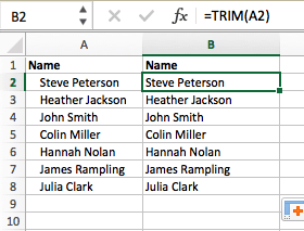
The TRIM formula in Excel is denoted =TRIM(text). This formula will remove any spaces entered before and after the text entered in the cell. For example, if A2 includes the name " Steve Peterson" with unwanted spaces before the first name, =TRIM(A2) would return "Steve Peterson" with no spaces in a new cell.

Email and file sharing are wonderful tools in today's workplace. That is, until one of your colleagues sends you a worksheet with some really funky spacing. Not only can those rogue spaces make it difficult to search for data, but they also affect the results when you try to add up columns of numbers.

Rather than painstakingly removing and adding spaces as needed, you can clean up any irregular spacing using the TRIM function, which is used to remove extra spaces from data (except for single spaces between words).

• The formula: =TRIM(text).
  • Text: The text or cell from which you want to remove spaces.

Here's an example of how we used the TRIM function to remove extra spaces before a list of names. To do so, we entered =TRIM("A2") into the Formula Bar, and replicated this for each name below it in a new column next to the column with unwanted spaces.

Below are some other Excel formulas you might find useful as your data management needs grow.

LEFT, MID, and RIGHT Formula

Let's say you have a line of text within a cell that you want to break down into a few different segments. Rather than manually retyping each piece of the code into its respective column, users can leverage a series of string functions to deconstruct the sequence as needed: LEFT, MID, or RIGHT.

LEFT:

• Purpose: Used to extract the first X numbers or characters in a cell.
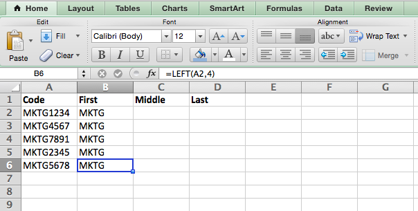
• The formula: =LEFT(text, number_of_characters)
  
  • Text: The string that you wish to extract from.
  • Number_of_characters: The number of characters that you wish to extract starting from the left-most character.

In the example below, we entered =LEFT(A2,4) into cell B2, and copied it into B3:B6. That allowed us to extract the first 4 characters of the code.

MID:

• Purpose: Used to extract characters or numbers in the middle based on position.
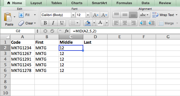
• The formula: =MID(text, start_position, number_of_characters)
  
  • Text: The string that you wish to extract from.
  • Start_position: The position in the string that you want to begin extracting from. For example, the first position in the string is 1.
  • Number_of_characters: The number of characters that you wish to extract.

In this example, we entered =MID(A2,5,2) into cell B2, and copied it into B3:B6. That allowed us to extract the two numbers starting in the fifth position of the code.

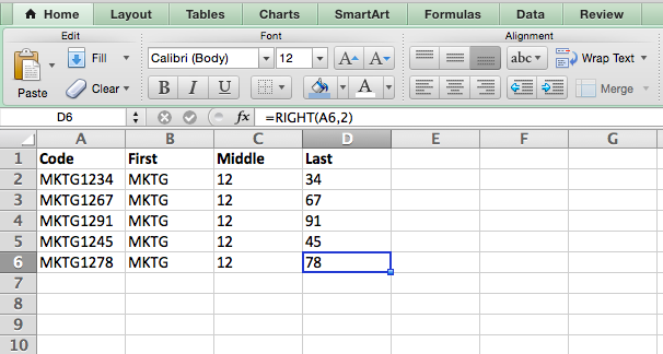
RIGHT:

• Purpose: Used to extract the last X numbers or characters in a cell.
• The formula: =RIGHT(text, number_of_characters)
  
  • Text: The string that you wish to extract from.
  • Number_of_characters: The number of characters that you want to extract starting from the right-most character.

For the sake of this example, we entered =RIGHT(A2,2) into cell B2, and copied it into B3:B6. That allowed us to extract the last two numbers of the code.

VLOOKUP Formula

This one is an oldie, but a goodie -- and it's a bit more in depth than some of the other formulas we've listed here. But it's especially helpful for those times when you have two sets of data on two different spreadsheets, and want to combine them into a single spreadsheet.

My colleague, Rachel Sprung -- whose "How to Use Excel" tutorial is a must-read for anyone who wants to learn -- uses a list of names, email addresses, and companies as an example. If you have a list of people's names next to their email addresses in one spreadsheet, and a list of those same people's email addresses next to their company names in the other, but you want the names, email addresses, and company names of those people to appear in one place -- that's where VLOOKUP comes in.

Note: When using this formula, you must be certain that at least one column appears identically in both spreadsheets. Scour your data sets to make sure the column of data you're using to combine your information is exactly the same, including no extra spaces.

• The formula: VLOOKUP(lookup value, table array, column number, [range lookup])
  • Lookup Value: The identical value you have in both spreadsheets. Choose the first value in your first spreadsheet. In Sprung's example that follows, this means the first email address on the list, or cell 2 (C2).
  • Table Array: The range of columns on Sheet 2 you're going to pull your data from, including the column of data identical to your lookup value (in our example, email addresses) in Sheet 1 as well as the column of data you're trying to copy to Sheet 1. In our example, this is "Sheet2!A:B." "A" means Column A in Sheet 2, which is the column in Sheet 2 where the data identical to our lookup value (email) in Sheet 1 is listed. The "B" means Column B, which contains the information that's only available in Sheet 2 that you want to translate to Sheet 1.
  • Column Number: The table array tells Excel where (which column) the new data you want to copy to Sheet 1 is located. In our example, this would be the "House" column, the second one in our table array, making it column number 2.
  • Range Lookup: Use FALSE to ensure you pull in only exact value matches.
• The formula with variables from Sprung's example below: =VLOOKUP(C2,Sheet2!A:B,2,FALSE)

In this example, Sheet 1 and Sheet 2 contain lists describing different information about the same people, and the common thread between the two is their email addresses. Let's say we want to combine both datasets so that all the house information from Sheet 2 translates over to Sheet 1. Here's how that would work:

RANDOMIZE Formula

There's a great article that likens Excel's RANDOMIZE formula to shuffling a deck of cards. The entire deck is a column, and each card -- 52 in a deck -- is a row. "To shuffle the deck," writes Steve McDonnell, "you can compute a new column of data, populate each cell in the column with a random number, and sort the workbook based on the random number field."

In marketing, you might use this feature when you want to assign a random number to a list of contacts -- like if you wanted to experiment with a new email campaign and had to use blind criteria to select who would receive it. By assigning numbers to said contacts, you could apply the rule, “Any contact with a figure of 6 or above will be added to the new campaign.”

• The formula: RAND()
  • Start with a single column of contacts. Then, in the column adjacent to it, type “RAND()” -- without the quotation marks -- starting with the top contact’s row.
• For the example below: RANDBETWEEN(bottom,top)
  • RANDBETWEEN allows you to dictate the range of numbers that you want to be assigned. In the case of this example, I wanted to use one through 10.
  • bottom: The lowest number in the range.
  • top: The highest number in the range,
• Formula in below example: =RANDBETWEEN(1,10)

Helpful stuff, right? Now for the icing on the cake: Once you've mastered the Excel formula you need, you'll want to replicate it for other cells without rewriting the formula. And luckily, there's an Excel function for that, too. Check it out below.

How to Copy Formula in Excel

1. Type your formula into an empty cell.
2. Press "Enter" to run the formula.
3. Hover your cursor over the bottom-right corner of the cell containing the formula.
4. Click and hold the small plus ("+") sign that appears.
5. Drag your cursor down the column.
6. Release your mouse to copy the formula into each subsequent cell.
7. Check each new value to ensure it corresponds to the correct cells.

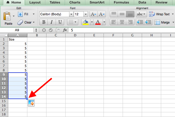
Tired of manually entering data that follows a pattern across a bunch of cells? Excel's Auto Fill feature is designed to minimize the work required on your end, by making it easy to repeat values you've already input.

To do so, click and hold the lower right corner of a cell, and then drag it down or across into adjacent cells. When you release, Excel will fill in the adjacent cells with the data from the cell you first selected.

Excel Keyboard Shortcuts

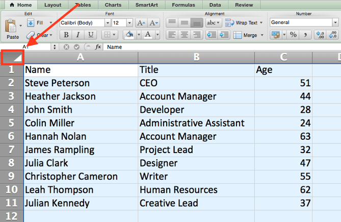
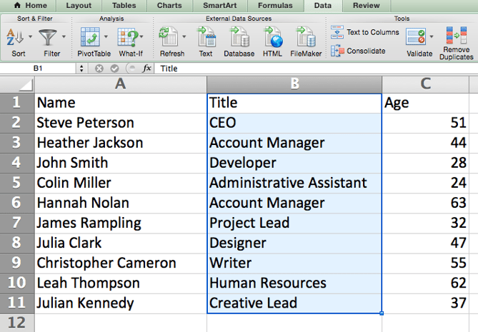
Quickly select rows, columns, or the whole spreadsheet.

Perhaps you're crunched for time. I mean, who isn't? No time, no problem. You can select your entire spreadsheet in just one click. All you have to do is simply click the tab in the top-left corner of your sheet to highlight everything all at once.

Just want to select everything in a particular column of row? That's just as easy with these shortcuts:

For Mac:

• Select Column = Command + Shift + Down/Up
• Select Row = Command + Shift + Right/Left

For PC:

• Select Column = Control + Shift + Down/Up
• Select Row = Control + Shift + Right/Left

This shortcut is especially helpful when you're working with larger data sets, but only need to select a specific piece of it.

Quickly open, close, or create a workbook.

Need to open, close, or create a workbook on the fly? The following keyboard shortcuts will enable you to complete any of the above actions in less than a minute's time.

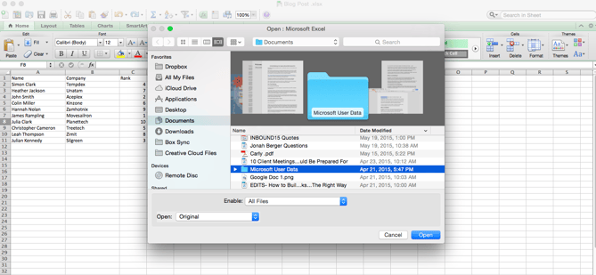
For Mac:

• Open = Command + O
• Close = Command + W
• Create New = Command + N

For PC:

• Open = Control + O
• Close = Control + F4
• Create New = Control + N

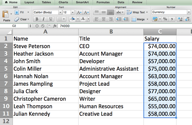
Format numbers into currency.

Have raw data that you want to turn into currency? Whether it be salary figures, marketing budgets, or ticket sales for an event, the solution is simple. Just highlight the cells you wish to reformat, and select Control + Shift + $.

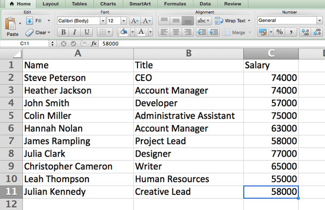
The numbers will automatically translate into dollar amounts -- complete with dollar signs, commas, and decimal points.

Note: This shortcut also works with percentages. If you want to label a column of numerical values as "percent" figures, replace "$" with "%".

Insert current date and time into a cell.

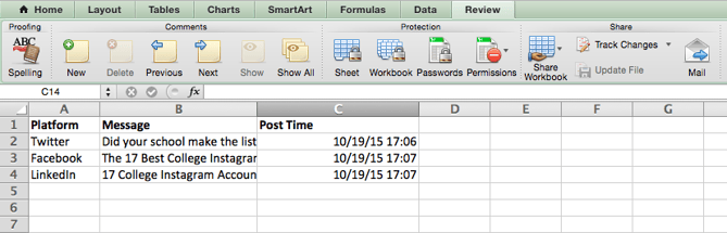
Whether you're logging social media posts, or keeping track of tasks you're checking off your to-do list, you might want to add a date and time stamp to your worksheet. Start by selecting the cell to which you want to add this information.

Then, depending on what you want to insert, do one of the following:

• Insert current date = Control + ; (semi-colon)
• Insert current time = Control + Shift + ; (semi-colon)
• Insert current date and time = Control + ; (semi-colon), SPACE, and then Control + Shift + ; (semi-colon).

Other Excel Tricks

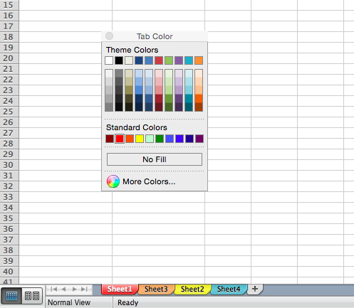
Customize the color of your tabs.

If you've got a ton of different sheets in one workbook -- which happens to the best of us -- make it easier to identify where you need to go by color-coding the tabs. For example, you might label last month's marketing reports with red, and this month's with orange.

Simply right click a tab and select "Tab Color." A popup will appear that allows you to choose a color from an existing theme, or customize one to meet your needs.

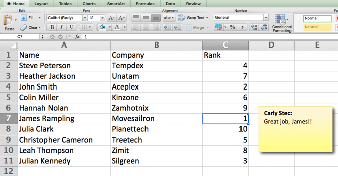
Add a comment to a cell.

When you want to make a note or add a comment to a specific cell within a worksheet, simply right-click the cell you want to comment on, then click Insert Comment. Type your comment into the text box, and click outside the comment box to save it.

Cells that contain comments display a small, red triangle in the corner. To view the comment, hover over it.

Copy and duplicate formatting.

If you've ever spent some time formatting a sheet to your liking, you probably agree that it's not exactly the most enjoyable activity. In fact, it's pretty tedious.

For that reason, it's likely that you don't want to repeat the process next time -- nor do you have to. Thanks to Excel's Format Painter, you can easily copy the formatting from one area of a worksheet to another.

Select what you'd like to replicate, then select the Format Painter option -- the paintbrush icon -- from the dashboard. The pointer will then display a paintbrush, prompting you to select the cell, text, or entire worksheet to which you want to apply that formatting, as shown below:

Identify duplicate values.

In many instances, duplicate values -- like duplicate content when managing SEO -- can be troublesome if gone uncorrected. In some cases, though, you simply need to be aware of it.

Whatever the situation may be, it's easy to surface any existing duplicate values within your worksheet in just a few quick steps. To do so, click into the Conditional Formatting option, and select Highlight Cell Rules > Duplicate Values

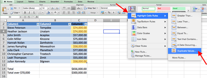
Using the popup, create the desired formatting rule to specify which type of duplicate content you wish to bring forward.

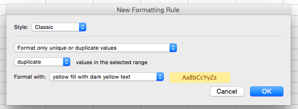
In the example above, we were looking to identify any duplicate salaries within the selected range, and formatted the duplicate cells in yellow.

In marketing, the use of Excel is pretty inevitable -- but with these tricks, it doesn't have to be so daunting. As they say, practice makes perfect. The more you use these formulas, shortcuts, and tricks, the more they'll become second nature.

To dig a little deeper, check out a few of our favorite resources for learning Excel. Want more Excel tips? Check out this post on how to create a pivot table with medians.

from Marketing https://blog.hubspot.com/marketing/excel-formulas-keyboard-shortcuts